With the latest GridOS challenge hosted on everybody.codes, I realised I skipped the last part of Quest 15 of the 2025 event. At the time this was due to the “Definitely Not a Maze” becoming too big for my BFS to solve, and I did not know a good way to solve it. I discovered from Reddit posts that most people used a technique called Coordinate Compression, which I had never heard of.
Looking it up did bring up a few articles of how to do it, but I wanted to understand it before doing so. I put it on hold then and picked it back up recently to dive more into the subject. This post describes the overall idea behind Coordinate Compression, how to do it, and then what I think was missing from other places; why it works.
Solving a big maze
The problem: Find the shortest path through the maze:
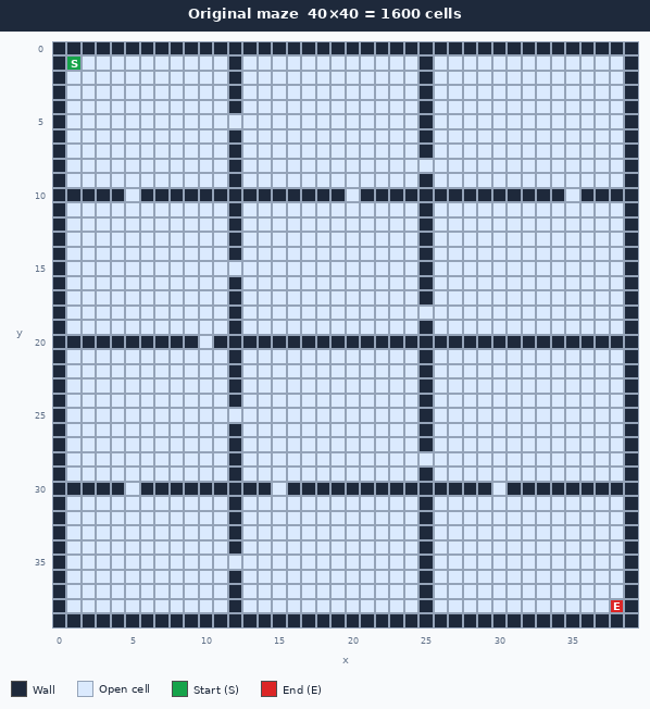
This can be easily solved by a Breadth-first search. In a 40×40 space it will not have any problems. However, BFS has to visit and remember every cell it reaches, so both its running time and its memory grow with the number of cells. Scale this same grid up 100 times or more and the search quickly becomes too slow and too memory-hungry to finish. This is hard to show in an image, which is why the illustrations will be of smaller graphs.
This maze in reality only consists of a few large zones separated by full-length walls, and each zone connects to its neighbour through a single narrow gap. This is very obvious to the human eye. Even if you scaled the whole maze up so each zone was ten times larger, there would still be only one gap between neighbouring zones (now just wider, with more possible ways through). The interior of each zone is what you can think of as empty space.
How to use Coordinate Compression
The idea is to use this empty space to form a new compressed graph, where the empty space is compressed into a smaller set of nodes. The compression is done by scanning the rows and then the columns and keeping a boundary wherever a row (or column) differs from the one before it. A run of identical rows collapses into a single compressed row, and the same is done for columns. (The “Why it works” section explains exactly which rows count as different, and why.) This can be seen in the following gif:
The gif shows the two graphs side by side. You can see that it produces a somewhat similar graph, but with a different ratio. This can also be illustrated as mapping the compressed coordinate boxes onto the original graph as seen in this image:
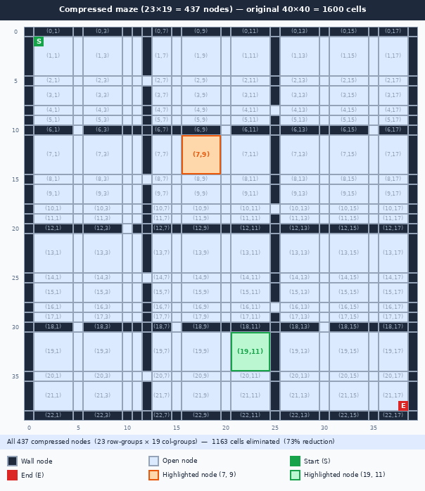
The highlighted areas are to show how regions of 3×3 original cells are grouped into a single compressed cell in the compressed graph. You might wonder why we split the zones so many times, and that will be discussed further in the “Why it works”-section.
In code this can be stored as two 1D arrays, one per axis, where each index is the compressed coordinate and the value is the corresponding original coordinate. The x and y axes are compressed independently, so a compressed position (cx, cy) maps back to the original position (xs[cx], ys[cy]). The distance between two neighbouring compressed cells is just the difference between their stored original coordinates, which is what gives each edge its weight later.
After this compression, Dijkstra’s algorithm can be run on the compressed graph to find the shortest path. The steps should still be counted using the lengths in the real graph, but the compressed graph can be used for finding the neighbours. The following gif helps to understand how the search through the compressed graph correlates to the original graph:
Why it works
Coordinate compression works because every position inside a compressed cell has the same neighbourhood structure. This is where the splitting described earlier becomes important. By introducing splits at every change in the maze’s layout (and around those changes), every compressed cell is guaranteed to contain only positions that behave identically. No matter where you are inside a compressed cell, you can only leave it through the same neighbouring compressed cells.
So why split around every change, and not just at the change itself? Consider a single column where a wall ends and an opening begins. The cells in that column are not all the same: the cell right next to the opening can step sideways through the gap, while the cells further along the wall cannot. If you grouped that whole column into one compressed cell, the group would contain positions with different escape routes, and the “you can only leave through the same neighbours” guarantee would break. To avoid this, you take every coordinate where something changes and also keep the coordinate on either side of it as its own row or column. In practice this means collecting the significant coordinates and, for each one c, splitting at c-1, c, and c+1 (where splits from neighbouring coordinates overlap, they simply collapse together).
This is also why you cannot simply make each zone its own box. A turn in the shortest path can only happen at a boundary, so the boundaries must survive compression as distinct cells. If the splits are too coarse, the compressed graph loses the ability to turn at the right place, and Dijkstra can no longer reconstruct the true shortest path.
The compression does not remove any possible routes through the maze. Instead, it groups large regions of equivalent cells into a single node while recording the real distances between neighbouring regions. A move in the compressed graph may therefore represent many steps in the original maze.
This is why Dijkstra’s algorithm is used instead of Breadth-first search. In the original maze every edge has a cost of 1, making BFS sufficient. After compression, edges can have different costs corresponding to the actual distance travelled in the original maze. The compressed graph is therefore a weighted graph, which is exactly the type of problem Dijkstra’s algorithm solves.
Coordinate compression removes coordinates, not geometry. Large empty regions are replaced by weighted rectangles that preserve both the available routes and the distance of those routes. Dijkstra does not care whether an edge represents one step or one thousand steps; it only requires that the edge weight reflects the true travel cost. Because the compressed graph preserves those costs, the shortest path found in the compressed graph is identical to the shortest path in the original maze.
Conclusion
In Quest 15 the compression was actually a lot simpler, since each move represented a coordinate break of c-1, c and c+1 around the the x and y of each wall end.
Writing up this article helped me better understand why this solves the problem. I think that by having an understanding of why it works, it becomes easier to apply to problems. Specifically, this only fits a graph with a huge empty space and would not make much sense in a denser maze. Additionally, you need more splits than I would initially have imagined. This does not work if you try to make each box its own, as then Dijkstra could not prove it was the shortest. I hope this helped you understand it too.